The danger of overfitting is one of the most important lessons of machine learning, a branch of artificial intelligence focused on building computer programs that can learn from data. The general concept of overfitting, however, has applications everywhere in life, and so I want to share it with you.
To do that, I’m going to teach you what overfitting means from a machine learning standpoint, convince you of its importance, and then ground the machine learning concept solidly in real life applications.
First, we start with some data. This could be information about tensile strengths of aircraft alloys, traffic patterns for self driving cars, or even the movements of the stock market—anything we want to be able to predict based on past observations.
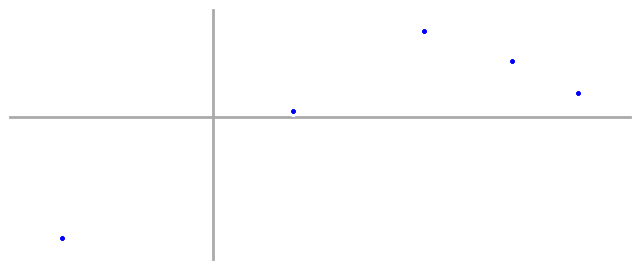
And a problem: given that these data points came from the same process, we want to predict what other data from the same process might look like.
In this case, we have five data points. Remembering our algebra, we realize that we can perfectly fit a fourth order polynomial with five points, so let’s do that, graph it, and see what we get.
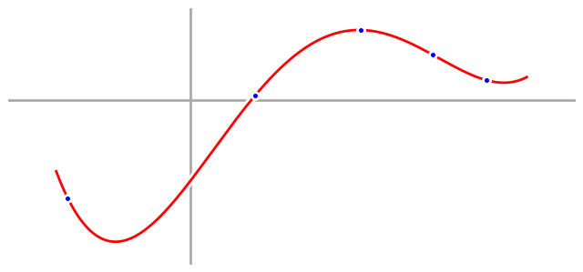
And it’s a perfect fit to our five data points. Really, we shouldn’t be surprised, because we knew that would happen. What will surprise us, though, is that when we take our fourth order model into the wild and use it to predict new data points, we do terribly. We’re wrong on almost everything, and as a result, the wings fall off our airplane, our self driving car crashes into a stop sign, and we lose all of our money when we bet on the stock market.
But we won’t be deterred.
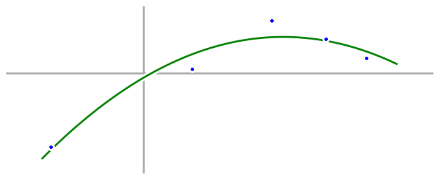
After our first failure, we come back again and try a new approach. Instead of taking our five data points and happily fitting them to a fourth order polynomial, we take a moment to just look at them and note what we see. This time, we’re thinking about Occam’s Razor—that the simplest explanation is often best—and so we decide that we want to find the simplest possible model that fits the main characteristics of the data. In our case, the data start low, go high, and then low again, so we decide to try fitting the data again, but this time we’ll fit it with a parabola, or second order polynomial, the simplest equation we can think of that can start low, go high, and then go low again. The cost we’ll pay is that we won’t be able to fit our data points exactly, but we can find the parabola that’s closest to all of them, and that’s what we do.
Now we take our new quadratic model—a quadratic equation and a parabola are the same thing—out into the real world, and we’re delighted to watch our airplanes fly, our self-driving cars navigate rush hour, and our bank account grow, as we finally beat the stock market.
So why didn’t the fourth order model work?
To understand why our first model didn’t work, let’s take a look at the actual process (aka - the equation behind the scene) that generated the data.
The first thing you should notice is that our data points don’t actually fall right on the generating equation. That’s because I added a little bit of randomness to each data point between generating it and displaying it for the first time. That randomness is called ‘noise’, and it appears everywhere: alloys have defects, people change lanes without warning, and sometimes someone hacks a news agency’s Twitter account and momentarily crashes the stock market by posting fake news.
Now let’s add our models to this graph and see directly how they stack up. First, our fourth order model:
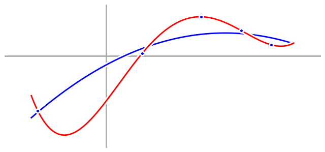
And we can clearly see how our fourth order model totally fails to match the process we were trying to model, despite fitting our data perfectly.
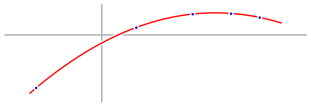
The problem is that in fitting our data perfectly, our fourth order model also fit the noise in our data perfectly, and that’s called overfitting. We say that we have overfit the data when the noise in the data causes our model to be a worse approximation of the underlying process. In this case, that little bit of randomness in the data threw our fourth order model totally off. To prove it, here’s what a fourth order fit would look like if our data didn’t have any noise.
That graph actually still has the blue process line on it, you just can’t see it because the red fourth order model overlaps it perfectly.
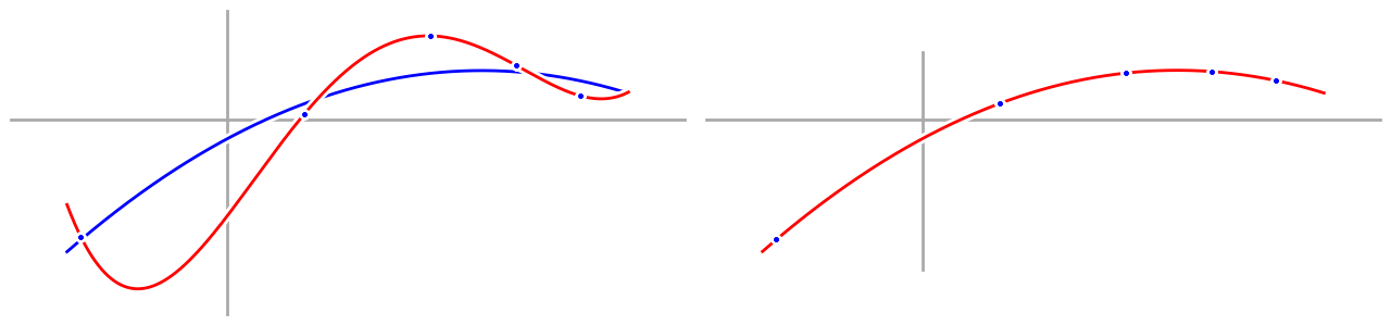
To really drive home my point, here are the two graphs again, side by side. A little bit of randomness makes everything go to hell when you require a perfect explanation.
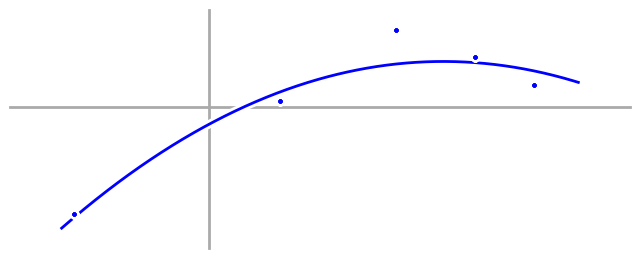
Now let’s take a look at our quadratic model:
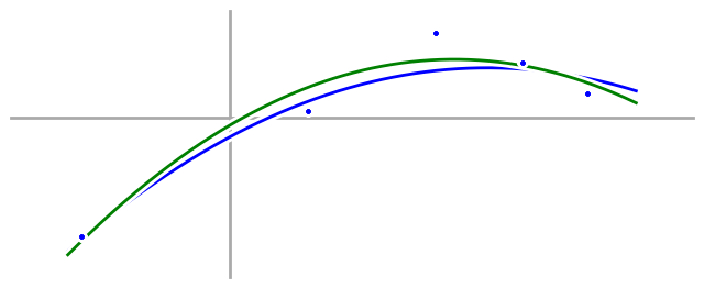
Compared to our fourth order model, our quadratic model doesn’t hit the data points exactly, but it matches the underlying process much better. The first part shouldn’t surprise us, after all, we have five data points and only three parameters in our quadratic model—of course we can’t fit the data exactly. Instead, we have to be satisfied with merely being close. But by satisfying ourselves with being close, we are, in essence, smoothing out the noise in our data, so our final quadratic model isn’t affected by the noise as much, and works much better.
What does this have to do with everyday life?
The trick is realizing that you can think of everything in your life—especially your interactions with other people!—like a source of data that you use to build mental models.
Let’s start with the case of people, and get specific. I want you to take a moment now, and think back to the last time that someone you know acted uncharacteristically assholeish. Your mental model of them probably took a hit. “Man, Alex sure is an asshole,” you thought. Psychologists call this the fundamental attribution error, and the problem is that when you look at Alex, you see his behavior, and you attribute it to his personality, in this case changing your mental model of Alex to include the fact that he’s an asshole.
But when was the last time that you acted like an asshole to someone? Did you happen to be tired, stressed out, or worried about something? Maybe they just caught you at the wrong time? Odds are, you understand that you’re not actually an asshole at heart, but just had a bad day. Those extra factors, the car alarms that kept you awake the night before, the painful ankle you twisted last weekend, and the argument you just had with your sister play the role of random noise that combines with your underlying personality to produce your behavior.
Perfectly reasonable people have bad days, and noisy data doesn’t always fit a line. When you demand a perfect explanation for everything, though, your models stop matching reality. You come to believe that Alex really is an asshole, and so you avoid events that he’s at, even though he’s usually the life of the party. Your incorrect models mean you miss out.
The moral of the story:
In life, work, and everything else, look for underlying trends, use simple explanations to understand your data, and try to ignore the noise. Accept the fact that perfect explanations are not only overrated, but dangerous. If you can satisfy yourself with merely good explanations, you’ll be much more accurate.
I’d like to thank Professor Yaser Abu-Mostafa of Caltech, and all of the staff who came together to offer his CS 156 - Machine Learning online course, where I had my my intuitive understanding of overfitting from physics grounded in concrete mathematics.
I’ve taken some liberties with the mathematical details behind overfitting in the intuitive explanation above. If you’d like to understand the details of the theory behind it, any many other related and exciting things, I highly recommend the CS 156 online course linked above.